library(tidyverse)
library(paramtest)How to do power simulations for structural equation models in R
R & Statistics
Open Science
Computing a priori power analyses for simple statistical models can be done analytically (e.g., with G*Power or the pwr package in R). However, estimating the power for more complex models and in particular structural…
Computing a priori power analyses for simple statistical models can be done analytically (e.g., with G*Power or the pwr package in R). However, estimating the power for more complex models and in particular structural equation models (SEM) is not as straightforward and requires simulations. I recently came across the package paramtest (Hughes, 2017) which provides a great framework for conducting more complex power simulations.
In what follows, I provide some examples of how to simulate power for SEMs with the ultimate goal of estimating the required sample size. On a side note, SEM are comparatively complex models. Sample size justifications are hence not only based on power calculations but should also be informed by general considerations of model complexity (see e.g., Kline, 2015).
For the following analyses, we only need two packages. I will use various functions from the tidyverse (primarily from dplyr and ggplot2) and the functions gen_data() and grid_search() from the paramtest package.
Helper functions: caching, power summaries and plot styling
# The simulations take a while. Their results are saved next to this post
# (folder sims/) and re-used; delete the files to run them again.
cached <- function(file, expr) {
  if (file.exists(file)) return(readRDS(file))
  dir.create(dirname(file), showWarnings = FALSE)
  res <- expr
  saveRDS(res, file)
  res
}

# Power per sample size, with a 95% (Wilson) interval for the Monte Carlo error
summarise_power <- function(data, significant) {
  data |>
    group_by(n = n.test) |>
    summarise(k = sum({{ significant }}, na.rm = TRUE),
              iter = sum(!is.na({{ significant }})),
              .groups = "drop") |>
    mutate(power = k / iter,
           z = qnorm(.975),
           centre = (power + z^2 / (2 * iter)) / (1 + z^2 / iter),
           halfw = z * sqrt(power * (1 - power) / iter + z^2 / (4 * iter^2)) / (1 + z^2 / iter),
           lower = centre - halfw, upper = centre + halfw) |>
    select(n, k, iter, power, lower, upper)
}

# A smooth power curve: power is approximately Phi(a + b * sqrt(n))
power_fit <- function(pw) glm(cbind(k, iter - k) ~ sqrt(n), family = binomial("probit"), data = pw)
n_for_power <- function(fit, target = .80) unname(((qnorm(target) - coef(fit)[1]) / coef(fit)[2])^2)
power_curve <- function(fit, n) tibble(n = n, power = predict(fit, tibble(n = n), type = "response"))
fmt_n <- function(n) format(round(n, -1), big.mark = ",")

# Plot style: transparent background, muted text (readable in light and dark mode)
pal <- c(blue = "#1497d6", orange = "#d9772b", green = "#1baf7a", grey = "#8a8f98")
theme_blog <- function() {
  theme_minimal(base_size = 12) +
    theme(plot.background  = element_rect(fill = "transparent", colour = NA),
          panel.background = element_rect(fill = "transparent", colour = NA),
          panel.grid.minor = element_blank(),
          panel.grid.major = element_line(colour = "#8a8f9840", linewidth = .4),
          axis.text  = element_text(colour = "#7a7f88"),
          axis.title = element_text(colour = "#7a7f88"),
          legend.position = "none")
}
Power for a bivariate relationship with manifest variables
Let us first consider a simple bivariate relationship between two manifest variables. In other words, we investigate the power for a relationship between two variables with “no measurement error”. The approach that I am going to use throughout this post is always as follows:
- Define a function that simulates data, draw samples, estimate the relevant models, and extract parameters of interest.
- Use
grid_search()to run the simulations. - Count the number of significant results to “get” power.
- Visualize the power curve.
The first step requires defining a function with the following arguments: a) simNum = the iteration number (do not change this argument, it is required by grid_search()), b) n = the sample sizes that should be tests, c) any other variables that should vary across the simulations (could be effect size(s) of the relationship(s) of interest or factor loadings of latent variables, etc.). Within this function, we use the function gen_data() that generates samples from the predefined data properties.
These properties include a “factor matrix” and an “effect matrix”. Defining both matrixes requires a good knowledge about the model that one wants to estimate. All steps are outlined below.
# Define the function
model_bivar <- function(simNum, n, b1) {

  # compute factor matrix
  factor <- matrix(c(1, 0,    # x (no measurement error)
                     0, 1),   # y (no measurement error)
                   nrow = 2, ncol = 2,
                   byrow = TRUE,
                   dimnames = list(c('x', 'y'),  # rows
                                   c('x', 'y'))) # cols
  # compute effect matrix
  y_res <- sqrt(1 - b1^2)
  effect <- matrix(c(1, b1,    # b1 = effect size of the relationship
                     0, y_res),
                    nrow = 2, ncol = 2,
                    byrow = TRUE,
                    dimnames = list(c('x', 'y'),    # rows
                                    c('x', 'y')))   # columns

  # generate data based on both matrices
  data <- paramtest::gen_data(factor, effect, n_cases = n)

  # fit lavaan model
  model <- '
    y ~ b1*x
  '
  fit <- lavaan::sem(model, data = data)

  # extract relevant parameters
  ests <- subset(lavaan::parameterEstimates(fit), label == "b1")
  return(ests)
}
Now, we use grid_search() to run the simulations. In this case, we investigate how many participants we need to sample in order to test a bivariate effect between manifest variables of \(\beta\) = .10 (small according to Cohen) to reach different levels of power.
We hence provide a list with the varying parameters (in this case only the sample sizes). It is important to run enough iterations. As always, results stabilize with higher iterations. Side note: We can profit from parallel computing by using parallel = 'snow' and ncpus = [number of available cores]. This increases the computation speed considerably.
# Run simulations (L'Ecuyer-CMRG makes the parallel random numbers reproducible)
RNGkind("L'Ecuyer-CMRG")
set.seed(2020)
power_bivar <- cached("sims/power_bivar.rds", grid_search(
  func = model_bivar,
  params = list(n = seq(100, 1500, by = 50)),
  b1 = .1,
  n.iter = 1000,
  output = 'data.frame',
  parallel = 'snow',
  ncpus = parallel::detectCores() - 1
  ))
# result table
results(power_bivar) %>% as_tibble#> # A tibble: 29,000 × 12
#> iter n.test lhs op rhs label est se z pvalue ci.lower
#> <int> <dbl> <chr> <chr> <chr> <chr> <dbl> <dbl> <dbl> <dbl> <dbl>
#> 1 1 100 y ~ x b1 0.0640 0.0990 0.646 0.518 -0.130
#> 2 2 100 y ~ x b1 0.160 0.0994 1.61 0.107 -0.0345
#> 3 3 100 y ~ x b1 0.0697 0.0970 0.718 0.473 -0.121
#> 4 4 100 y ~ x b1 0.175 0.106 1.65 0.0998 -0.0334
#> 5 5 100 y ~ x b1 -0.0444 0.0952 -0.467 0.641 -0.231
#> 6 6 100 y ~ x b1 0.182 0.106 1.72 0.0851 -0.0251
#> 7 7 100 y ~ x b1 0.184 0.0907 2.03 0.0425 0.00621
#> 8 8 100 y ~ x b1 0.0676 0.110 0.616 0.538 -0.147
#> 9 9 100 y ~ x b1 0.115 0.102 1.12 0.261 -0.0856
#> 10 10 100 y ~ x b1 -0.0108 0.0941 -0.115 0.908 -0.195
#> # ℹ 28,990 more rows
#> # ℹ 1 more variable: ci.upper <dbl>The resulting data frame includes relevant parameters for the relationship between x and y. The column n.test indicates the sample size of each iteration.
To compute the power, we only need to count the number of significant results per sample size group (n = 100, 150, 200, 250,…). We can then check the “needed” sample size for various power levels. It would also suggest plotting a power curve as it provides more information than a single value alone.
# compute power
(result_bivar <- results(power_bivar) %>%
  group_by(n.test) %>%
  mutate(sig = (pvalue < .05)) %>%
  summarise(power = mean(sig, na.rm=TRUE)))
#> # A tibble: 29 × 2
#> n.test power
#> <dbl> <dbl>
#> 1 100 0.171
#> 2 150 0.235
#> 3 200 0.311
#> 4 250 0.337
#> 5 300 0.415
#> 6 350 0.462
#> 7 400 0.552
#> 8 450 0.58
#> 9 500 0.614
#> 10 550 0.664
#> # ℹ 19 more rows# Extract sample size for 80% power
result_bivar %>%
filter(power >= 0.80)#> # A tibble: 15 × 2
#> n.test power
#> <dbl> <dbl>
#> 1 800 0.802
#> 2 850 0.826
#> 3 900 0.866
#> 4 950 0.872
#> 5 1000 0.887
#> 6 1050 0.895
#> 7 1100 0.921
#> 8 1150 0.941
#> 9 1200 0.942
#> 10 1250 0.944
#> 11 1300 0.959
#> 12 1350 0.963
#> 13 1400 0.96
#> 14 1450 0.97
#> 15 1500 0.979To plot a power curve, I add two things to the raw proportions: a 95% confidence interval for each estimate (with 1,000 iterations, the Monte Carlo error is about ±3 percentage points) and a smooth curve. Because power is approximately \(\Phi(a + b\sqrt{n})\), a probit regression on \(\sqrt{n}\) fits these curves very well, and we can solve it for the sample size that reaches 80% power.
# Power with Monte Carlo intervals, fitted curve and the n for 80% power
pw_bivar  <- summarise_power(results(power_bivar), pvalue < .05)
fit_bivar <- power_fit(pw_bivar)
n80_bivar <- n_for_power(fit_bivar)ggplot(pw_bivar, aes(n, power)) +
geom_hline(yintercept = .80, linetype = "dashed", colour = pal["grey"]) +
annotate("segment", x = n80_bivar, xend = n80_bivar, y = 0, yend = .80,
linetype = "dotted", colour = pal["grey"]) +
geom_line(data = power_curve(fit_bivar, 100:1500), colour = pal["blue"], linewidth = 1) +
geom_pointrange(aes(ymin = lower, ymax = upper), colour = pal["blue"], size = .2) +
annotate("text", x = n80_bivar + 30, y = .74, hjust = 0, colour = "#7a7f88",
label = paste0("80% power at n ≈ ", fmt_n(n80_bivar))) +
scale_y_continuous(labels = scales::percent, limits = c(0, 1)) +
labs(x = "Sample size", y = "Power") +
theme_blog()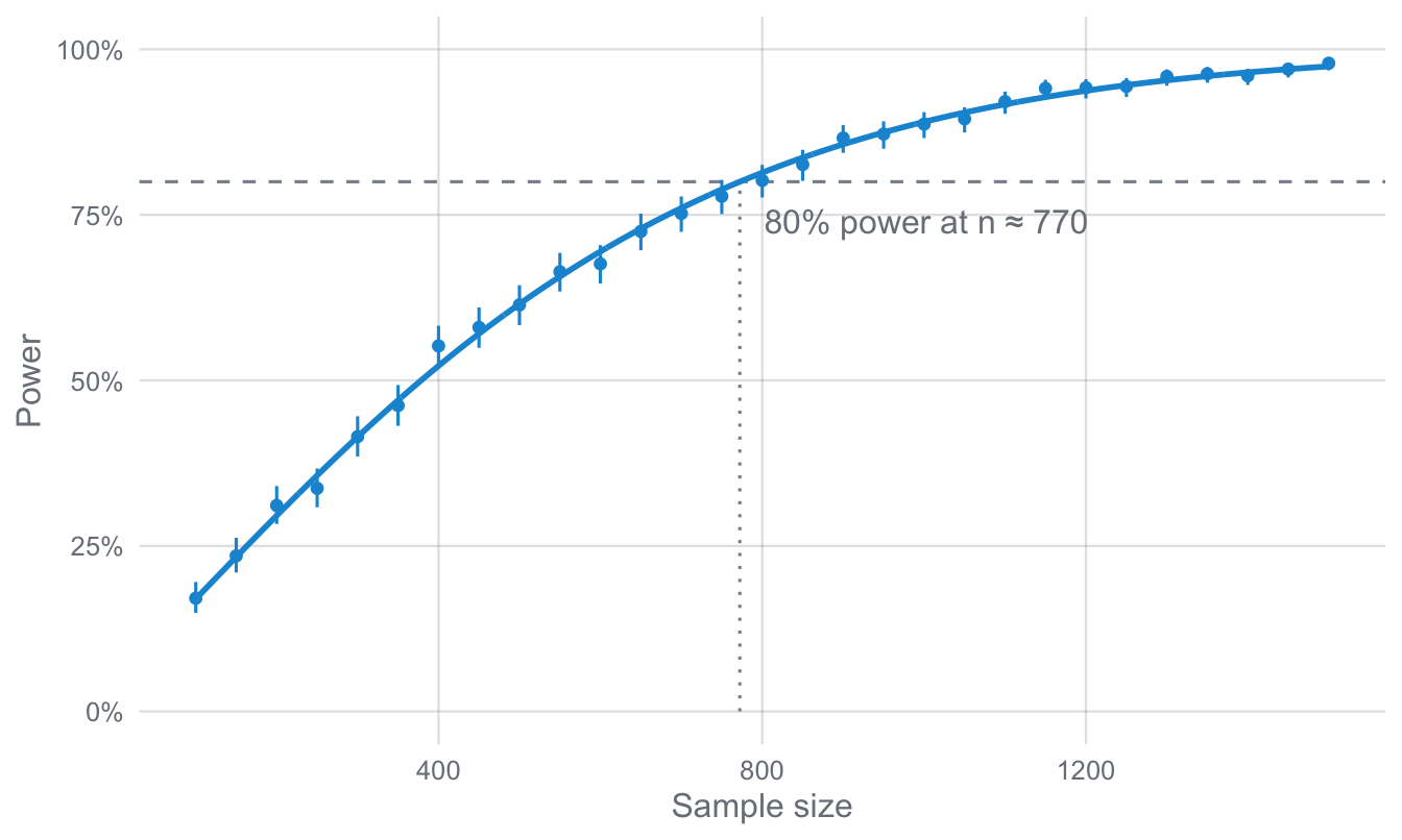
In this example, we see that we need roughly 770 participants in order to test the small correlation between the two variables with a power of 80% (assuming an alpha-level of .05!).
For this simple example, this procedure is a bit complex as a solution can also be derived analytically (any remaining difference in the resulting sample size is explainable by the Monte Carlo error of our simulations. With more iterations, we would get even closer to the analytical solution):
library(pwr)
pwr.r.test(r = c(.1),
           sig.level = .05,
           power = .80,
           alternative = "two.sided")
#>
#> approximate correlation power calculation (arctangh transformation)
#>
#> n = 781.7516
#> r = 0.1
#> sig.level = 0.05
#> power = 0.8
#> alternative = two.sidedPower for a bivariate relationship between latent variables
The whole procedure becomes more complex if we try to simulate the power for a relationship between latent variables. Here, we need to make assumptions about the items’ reliability. In this first example, we assume that we have comparatively good scales whose items have factor loadings of .70 (i.e., each item’s reliability is .70² = .49, and the reliability of a three-item scale is ω ≈ .74). Defining the factor matrix is hence more complex and the model is now a structural equation model with latent variables. Otherwise, the procedure remains the same.
# define function
model_sem <- function(simNum,
                      n,
                      b1,
                      x_ind1, x_ind2, x_ind3,
                      y_ind1, y_ind2, y_ind3) {

  # compute factor matrix (in this case with measurement error)
  factor <- matrix(c(x_ind1, 0,   # y1
                     x_ind2, 0,   # y2
                     x_ind3, 0,   # y3
                     0, y_ind1,   # y1
                     0, y_ind2,   # y2
                     0, y_ind3),  # y3
                   nrow=6, ncol=2,
                   byrow=TRUE,
                   dimnames=list(c('x1', 'x2', 'x3', 'y1', 'y2', 'y3'),  # rows (observed)
                                 c('x', 'y')))                           # columns (latent)

  # matrix of the effects structure (variance-covariance)
  y_res <- sqrt(1 - b1^2)
  effect <- matrix(c(1, b1,     # x
                     0, y_res), # y
                    nrow=2, ncol=2,
                    byrow=TRUE,
                    dimnames=list(c('x', 'y'),    # rows
                                  c('x', 'y')))   # columns

  # generate data based on both matrices
  data <- paramtest::gen_data(factor, effect, n_cases = n)

  # fit lavaan model
  model <- '
   # measurement model
   x =~ x1 + x2 + x3
   y =~ y1 + y2 + y3

   # structural regression model
   y ~ b1*x
  '
  fit <- lavaan::sem(model, data = data)
  ests <- lavaan::parameterEstimates(fit)

  # extract relevant parameters
  est <- ests[ests$label == 'b1', 'est']
  p <- ests[ests$label == 'b1', 'pvalue']
  return(c(est = est,
           p = p,
           sig = (p < .05)))
}

# Measurement error specified by factor loading = .7
RNGkind("L'Ecuyer-CMRG")
set.seed(2021)
power_sem1 <- cached("sims/power_sem1.rds", grid_search(
  func = model_sem,
  params = list(n = seq(500, 4000, by = 100)),
  b1 = .1,
  n.iter = 1000,
  output = 'data.frame',
  x_ind1 = .7,
  x_ind2 = .7,
  x_ind3 = .7,
  y_ind1 = .7,
  y_ind2 = .7,
  y_ind3 = .7,
  parallel = 'snow',
  ncpus = parallel::detectCores() - 1
  ))
Let us quickly check the resulting data frame.
results(power_sem1) %>% as_tibble#> # A tibble: 36,000 × 5
#> iter n.test est p sig
#> <int> <dbl> <dbl> <dbl> <dbl>
#> 1 1 500 0.00710 0.906 0
#> 2 2 500 0.182 0.0111 1
#> 3 3 500 0.165 0.00259 1
#> 4 4 500 0.0111 0.866 0
#> 5 5 500 0.142 0.00922 1
#> 6 6 500 0.111 0.110 0
#> 7 7 500 0.0879 0.168 0
#> 8 8 500 0.169 0.0112 1
#> 9 9 500 0.109 0.0469 1
#> 10 10 500 0.126 0.0396 1
#> # ℹ 35,990 more rowsThis time, we only extracted the estimate, the p-value, and already transformed the p-value into a binary variable (p < .05). Replications in which the model does not converge return NA and are dropped when we compute power (na.rm = TRUE).
But before we estimate the power, let us quickly run the simulation again, but change the reliability of the items to more realistic values (at least in the social sciences, scales often have items with factor loadings around .50). This is very easy, as the defined function has arguments for each factor loading in the model.
We then combine the results from both simulations. After a bit of data wrangling, we can now plot both power curves.
# Let's also test a more realistic example (factor loadings = .5)
set.seed(2022)
power_sem2 <- cached("sims/power_sem2.rds", grid_search(
  func = model_sem,
  params = list(n = seq(500, 4000, by = 100)),
  b1 = .1,
  n.iter = 1000,
  output = 'data.frame',
  x_ind1 = .5,    # changed to .5
  x_ind2 = .5,
  x_ind3 = .5,
  y_ind1 = .5,
  y_ind2 = .5,
  y_ind3 = .5,
  parallel = 'snow',
  ncpus = parallel::detectCores() - 1
  ))
# Extract result table
(result_sem1 <- results(power_sem1) %>%
mutate(rel = .7) %>%
bind_rows(results(power_sem2) %>%
mutate(rel = .5)) %>%
group_by(rel, n.test) %>%
summarise(power=mean(sig, na.rm=TRUE)))#> # A tibble: 72 × 3
#> # Groups: rel [2]
#> rel n.test power
#> <dbl> <dbl> <dbl>
#> 1 0.5 500 0.175
#> 2 0.5 600 0.192
#> 3 0.5 700 0.232
#> 4 0.5 800 0.3
#> 5 0.5 900 0.301
#> 6 0.5 1000 0.346
#> 7 0.5 1100 0.363
#> 8 0.5 1200 0.4
#> 9 0.5 1300 0.419
#> 10 0.5 1400 0.441
#> # ℹ 62 more rowspw_sem <- bind_rows(
summarise_power(results(power_sem1), sig == 1) |> mutate(loadings = ".70"),
summarise_power(results(power_sem2), sig == 1) |> mutate(loadings = ".50"))
fits_sem <- lapply(split(pw_sem, pw_sem$loadings), power_fit)
n80_sem <- sapply(fits_sem, n_for_power)
curves_sem <- bind_rows(lapply(names(fits_sem), \(l) power_curve(fits_sem[[l]], 500:4000) |> mutate(loadings = l)))ggplot(pw_sem, aes(n, power, colour = loadings)) +
geom_hline(yintercept = .80, linetype = "dashed", colour = pal["grey"]) +
geom_line(data = curves_sem, linewidth = 1) +
geom_pointrange(aes(ymin = lower, ymax = upper), size = .2) +
annotate("text", x = 4000, y = c(.20, .12), hjust = 1, colour = pal[c("blue", "orange")],
label = c("loadings .70 (ω ≈ .74)", "loadings .50 (ω = .50)")) +
scale_colour_manual(values = c(".70" = pal[["blue"]], ".50" = pal[["orange"]])) +
scale_y_continuous(labels = scales::percent, limits = c(0, 1)) +
labs(x = "Sample size", y = "Power") +
theme_blog()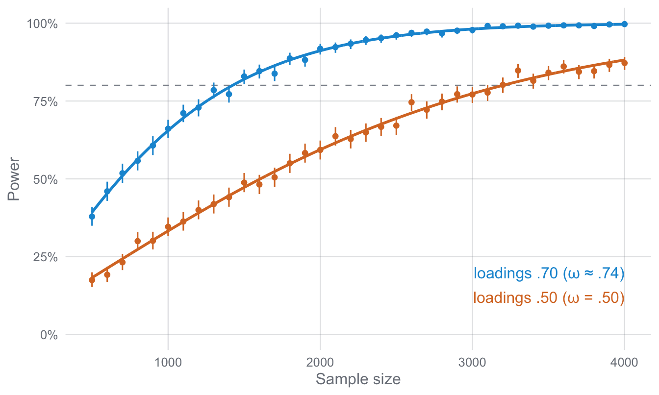
We can see two very interesting things in this plot: First, a small correlation between two latent variables requires a LOT more participants than the same correlation between manifest variables (of course: There is no measurement error in the model). But the difference is considerable depending on the items’ reliability. Whereas factor loadings of .70 already require more participants to reach a power of 80% (roughly 1,420 compared to 770 in the first example), reducing factor loadings to .50 (the more realistic scenario; the scale reliability then drops to ω = .50) requires about 3,200 (!!!) participants to reach a power of 80%.
Power for a simple mediation model with latent variables
At last, let us consider a simple mediation model with latent variables. Again, the procedure remains the same, only the factor and effect matrix needs to be defined correctly (I again assumed good scales with factor loadings of .70). Likewise, the SEM needs to be specified correctly and the parameters of interest need to be extracted. Interestingly, we can also compute the power to detect the indirect or total effect even though we may only have assumptions about the direct paths in the model!
model_med <- function(simNum,
                      n,
                      b1,
                      b2,
                      b3,
                      x_ind1, x_ind2, x_ind3,
                      m_ind1, m_ind2,
                      y_ind1, y_ind2, y_ind3) {

  # compute factor matrix (in this case with measurement error)
  factor <- matrix(c(x_ind1, 0, 0,   # x1
                     x_ind2, 0, 0,   # x2
                     x_ind3, 0, 0,   # x3
                     0, m_ind1, 0,   # m1
                     0, m_ind2, 0,   # m2
                     0, 0, y_ind1,   # y1
                     0, 0, y_ind2,   # y2
                     0, 0, y_ind3),  # y3
                   nrow=8, ncol=3,
                   byrow=TRUE,
                   dimnames=list(c('x1', 'x2', 'x3', 'm1', 'm2', 'y1', 'y2', 'y3'),  # rows (observed)
                                 c('x', 'm', 'y')))                           # columns (latent)

  # matrix of the effects structure: gen_data() computes latent = Z %*% effect,
  # with Z independent standard normal. To get m = b1*x + e_m and
  # y = b2*x + b3*m + e_y (all latent variances = 1), the weights must be:
  m_res <- sqrt(1 - b1^2)          # m's own (residual) part
  y_x   <- b2 + b1 * b3            # weight of x in y = direct + indirect effect
  y_m   <- b3 * m_res              # weight of m's residual part in y
  y_res <- sqrt(1 - y_x^2 - y_m^2) # y's own (residual) part
  effect <- matrix(c(1, b1,    y_x,   # x
                     0, m_res, y_m,   # m
                     0, 0,     y_res),# y
                    nrow=3, ncol=3,
                    byrow=TRUE,
                    dimnames=list(c('x', 'm', 'y'),    # rows
                                  c('x', 'm', 'y')))   # columns

  # generate data based on both matrices
  data <- paramtest::gen_data(factor, effect, n_cases = n)

  # fit lavaan model
  model <- '
   # measurement model
   x =~ x1 + x2 + x3
   y =~ y1 + y2 + y3
   m =~ m1 + m2

   # structural regression model
   m ~ b1*x
   y ~ b2*x + b3*m

   ind := b1*b3
   total := b2 + ind
  '
  fit <- lavaan::sem(model, data = data)
  ests <- lavaan::parameterEstimates(fit)

  # extract relevant parameters
  b1_est     <- ests[ests$label == 'b1', 'est']
  b1_p       <- ests[ests$label == 'b1', 'pvalue']
  b2_est     <- ests[ests$label == 'b2', 'est']
  b2_p       <- ests[ests$label == 'b2', 'pvalue']
  b3_est     <- ests[ests$label == 'b3', 'est']
  b3_p       <- ests[ests$label == 'b3', 'pvalue']
  ind_est    <- ests[ests$label == 'ind', 'est']
  ind_p      <- ests[ests$label == 'ind', 'pvalue']
  total_est  <- ests[ests$label == 'total', 'est']
  total_p    <- ests[ests$label == 'total', 'pvalue']

  return(c(b1_est   = b1_est,    b1_p    = b1_p,
           b2_est   = b2_est,    b2_p    = b2_p,
           b3_est   = b3_est,    b3_p    = b3_p,
           ind_est  = ind_est,   ind_p   = ind_p,
           total_est= total_est, total_p = total_p))
}

RNGkind("L'Ecuyer-CMRG")
set.seed(2023)
power_med <- cached("sims/power_med.rds", grid_search(
  func = model_med,
  params = list(n = seq(700, 4500, by = 100)),
  b1 = .1,  # assuming a small effect for all three paths
  b2 = .1,
  b3 = .1,
  n.iter = 1000,
  output = 'data.frame',
  x_ind1 = .7,
  x_ind2 = .7,
  x_ind3 = .7,
  m_ind1 = .7,
  m_ind2 = .7,
  y_ind1 = .7,
  y_ind2 = .7,
  y_ind3 = .7,
  parallel = 'snow',
  ncpus = parallel::detectCores() - 1
  ))
# Extract result table
(result_med <- results(power_med) %>%
group_by(n.test) %>%
mutate(b1_sig = (b1_p < .05),
b2_sig = (b2_p < .05),
b3_sig = (b3_p < .05),
ind_sig = (ind_p < .05),
total_sig = (total_p < .05)) %>%
summarise(b1_power = mean(b1_sig, na.rm=TRUE),
b2_power = mean(b2_sig, na.rm=TRUE),
b3_power = mean(b3_sig, na.rm=TRUE),
ind_power = mean(ind_sig, na.rm=TRUE),
total_power = mean(total_sig, na.rm=TRUE)))#> # A tibble: 39 × 6
#> n.test b1_power b2_power b3_power ind_power total_power
#> <dbl> <dbl> <dbl> <dbl> <dbl> <dbl>
#> 1 700 0.401 0.505 0.405 0.0557 0.589
#> 2 800 0.423 0.564 0.404 0.0652 0.637
#> 3 900 0.485 0.592 0.489 0.0956 0.666
#> 4 1000 0.550 0.662 0.530 0.145 0.756
#> 5 1100 0.561 0.694 0.557 0.148 0.767
#> 6 1200 0.599 0.727 0.598 0.195 0.819
#> 7 1300 0.648 0.746 0.662 0.246 0.825
#> 8 1400 0.693 0.781 0.690 0.287 0.851
#> 9 1500 0.698 0.829 0.712 0.309 0.879
#> 10 1600 0.731 0.811 0.736 0.378 0.882
#> # ℹ 29 more rowspw_med <- results(power_med) |>
pivot_longer(ends_with("_p"), names_to = "effect", values_to = "p") |>
mutate(effect = sub("_p$", "", effect)) |>
group_by(effect) |>
group_modify(~ summarise_power(.x, p < .05)) |>
ungroup()
fits_med <- lapply(split(pw_med, pw_med$effect), power_fit)
n80_med <- sapply(fits_med, n_for_power)
curves_med <- bind_rows(lapply(names(fits_med), \(e) power_curve(fits_med[[e]], 700:4500) |> mutate(effect = e)))# Three direct paths in one colour, the indirect and total effect highlighted
type <- c(b1 = "direct", b2 = "direct", b3 = "direct", ind = "indirect", total = "total")
cols <- c(direct = pal[["blue"]], indirect = pal[["orange"]], total = pal[["green"]])
labs_med <- tibble(type = c("direct", "total", "indirect"),
label = c("direct paths a, b, c′", "total effect c′ + a × b", "indirect effect a × b"),
y = c(.30, .22, .14))
ggplot(mutate(pw_med, type = type[effect]), aes(n, power, colour = type, group = effect)) +
geom_hline(yintercept = .80, linetype = "dashed", colour = pal["grey"]) +
geom_line(data = mutate(curves_med, type = type[effect]), linewidth = .9) +
geom_pointrange(aes(ymin = lower, ymax = upper), size = .15, alpha = .6) +
geom_text(data = labs_med, aes(x = 4500, y = y, label = label, colour = type),
inherit.aes = FALSE, hjust = 1) +
scale_colour_manual(values = cols) +
scale_y_continuous(labels = scales::percent, limits = c(0, 1)) +
labs(x = "Sample size", y = "Power") +
theme_blog()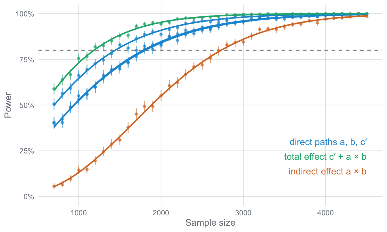
The result shows (as expected) that we need roughly the same sample size (about 1,440 to 1,810) to test the three direct paths in the model (as we assumed the same effect size of .10 for all three relationships). The path from x to m reaches 80% a bit earlier than the two paths into y, because the latter are estimated simultaneously (x and m are correlated) and the mediator is measured with only two indicators. However, we need considerably more participants to test the indirect effect (.10 × .10 = .01) with the same power! Here, we would need roughly 2,730 participants! Note that lavaan tests the indirect effect with the delta method (a Sobel-type test), which is known to be conservative. Bootstrapped or Monte Carlo confidence intervals have somewhat more power, but they are too slow to compute in every replication of a simulation like this one.
Conclusion
Simulating power for complex models is always going to be challenging due to the large number of parameters that one needs to make assumptions about. That said, the paramtest package provides a framework for doing so. In the examples above, I only varied the sample sizes. But I could have varied the effect sizes (or any other parameter in the simulation), too. This would allow analyzing the interaction between sample size and effect size on power to test such effects – from my point of view, this should be an important step before any study that aims at implementing structural equation modeling.
sessionInfo()#> R version 4.4.0 (2024-04-24)
#> Platform: aarch64-apple-darwin20
#> Running under: macOS 26.6.2
#>
#> Matrix products: default
#> BLAS: /Library/Frameworks/R.framework/Versions/4.4-arm64/Resources/lib/libRblas.0.dylib
#> LAPACK: /Library/Frameworks/R.framework/Versions/4.4-arm64/Resources/lib/libRlapack.dylib; LAPACK version 3.12.0
#>
#> Random number generation:
#> RNG: L'Ecuyer-CMRG
#> Normal: Inversion
#> Sample: Rejection
#>
#> locale:
#> [1] C.UTF-8/C.UTF-8/C.UTF-8/C/C.UTF-8/C.UTF-8
#>
#> time zone: Europe/Amsterdam
#> tzcode source: internal
#>
#> attached base packages:
#> [1] stats graphics grDevices utils datasets methods base
#>
#> other attached packages:
#> [1] pwr_1.3-0 paramtest_0.1.0 lubridate_1.9.3 forcats_1.0.0
#> [5] stringr_1.6.0 dplyr_1.2.0 purrr_1.2.1 readr_2.1.5
#> [9] tidyr_1.3.2 tibble_3.3.1 ggplot2_4.0.2 tidyverse_2.0.0
#>
#> loaded via a namespace (and not attached):
#> [1] gtable_0.3.6 jsonlite_2.0.0 compiler_4.4.0 tidyselect_1.2.1
#> [5] scales_1.4.0 yaml_2.3.12 fastmap_1.2.0 R6_2.6.1
#> [9] labeling_0.4.3 generics_0.1.4 knitr_1.51 htmlwidgets_1.6.4
#> [13] pillar_1.11.1 RColorBrewer_1.1-3 tzdb_0.4.0 rlang_1.1.7
#> [17] utf8_1.2.6 stringi_1.8.7 xfun_0.57 S7_0.2.1
#> [21] timechange_0.3.0 cli_3.6.5 withr_3.0.2 magrittr_2.0.4
#> [25] digest_0.6.39 grid_4.4.0 hms_1.1.3 lifecycle_1.0.5
#> [29] vctrs_0.7.2 evaluate_1.0.5 glue_1.8.0 farver_2.1.2
#> [33] rmarkdown_2.30 tools_4.4.0 pkgconfig_2.0.3 htmltools_0.5.8.1References
Hughes, J. (2017). paramtest: R package for varying parameters in simulations or other iterative processes. https://github.com/jeff-hughes/paramtest
Kline, R. (2015). Principles and Practice of Structural Equation Modeling. The Guilford Press.