What is ‘item sampling’ and why is it useful? Or how can we can measure person characteristics with large item pools?

I guess every social scientist at one point has been confronted with a quite common dilemma: We know that we would need a quite large number of items to assess a certain latent concept comprehensively and validly, but…

I guess every social scientist at one point has been confronted with a quite common dilemma: We know that we would need a quite large number of items to assess a certain latent concept comprehensively and validly, but we do not have enough space in our questionnaire to use the entire long scale or even inventory. More often than not, we then choose the “best” items (e.g., with the highest factor loadings). However, by reducing the number of items, we are likely reducing the scale’s validity as well. After all, we reduce the diversity and breadth of the manifest indicators that make up the scale.

An alternative to choosing a static subset of a scale that we administer to all participants in the exact same way is so-called item sampling. Here, the idea is to randomly select a subset of items for each respondent from a larger pool. This way, each participant answers a different subset of items. Due to the randomness in this sampling procedure, we can still gather sufficient information overall to estimate the latent trait for each individual participant. The question is, however, how many missing items per person are acceptable? And to what extent does the quality of the resulting scores depend on the size of the item pool, the size of the sample, and the original quality of the scale (e.g., as expressed by reliability indices such as Cronbach’s alpha)?

Statistical background

Classical Test Theory (CTT) offers a framework where each observed score (\(X\)) is conceptualized as the sum of a true score (\(T\)) and the error score (\(e\)):

\[X = T + e\]

In this context, the true score represents the actual level of the latent trait, and the error score encompasses all item-specific variance, measurement errors, or random noise.

CTT defines reliability as the proportion of variance in the observed scores that is attributable to the true scores. When items are randomly sampled, reliability can still be maintained by ensuring that the items are representative of the entire item pool and that the sampling process introduces minimal bias. The basic idea of item sampling is thus as follows:

• Random Selection of Items: Instead of administering the entire set of items (or a fixed subset) to every respondent, a small, randomly selected subset is given to each respondent, resulting in unique short scales per participant. This reduces the burden on respondents and shortens the questionnaire.
• Scoring with planned missing data: Because the items are missing completely at random (by design), we can estimate each person’s score from the items they answered, for example with a measurement model estimated by full information maximum likelihood (FIML). Alternatively, the unadministered items can be imputed. As we will see below, the first option is clearly preferable.

Despite the reduction in the number of items per respondent, the randomness and overlap between different respondents’ subsets ensure that the overall information about the latent trait is preserved at the level of the sample (e.g., means, variances, and correlations of the scale). For each individual person, however, the precision of their score depends on how many items they answered, as the following sections show.

Mathematical derivation

Given a large item pool, if we denote the total number of items by \(k\) and the number of items sampled for each respondent by \(k_s\), the reliability of the item-sampled test can be approximated by the Spearman-Brown prophecy formula (see e.g., de Vet et al., 2017)

\[\alpha_{new} = \frac{n*\alpha}{1+(n-1)*\alpha}\]

where:

• \(\alpha_{new}\) is the “new” reliability after item sampling
• \(n = k_s/k\) is the ratio of sampled items to total items
• \(\alpha\) is the original reliability of the full item pool

By ensuring \(k_s/k\) is sufficiently large, the reliability of the scale can be preserved to a certain degree. But how large should these two parameters be? Let’s compute the reliability after sampling 5 items from a pool of 10 given an alpha of .9:

# Set parameters
alpha <- .9
k_s <- 5
k <- 10

# Formula from above
new_alpha <- ((k_s/k)*alpha)/(1+((k_s/k)-1)*alpha)
round(new_alpha, 2)

#> [1] 0.82

As we can see, the resulting reliability is still .82 (compared to the original .90), which may be completely sufficient for some contexts. Now, let’s explore the relationship between the ratio of sampled to total items and alpha more systematically. Yet, so far, we did not account for the impact of sample size. Further, the above formula only tells us whether the reliability can be preserved. What we also would like to know is whether the validity is preserved (e.g., whether the correlation between the short and the full scale is large).

The impact of sample size can be included by considering the standard error of the reliability estimate and the standard error of the correlation. Larger sample sizes typically result in more precise estimates. For \(k_s\) (essentially) parallel items, the standard error of Cronbach’s alpha is approximately (van Zyl, Neudecker, & Nel, 2000):

\[SE_{\alpha} \approx (1-\alpha)\sqrt{\frac{2k_s}{(k_s-1)N}}\]

where:

• \(\alpha\) is the reliability of the reduced scale
• \(k_s\) is the number of items in the reduced scale
• \(N\) is the sample size

For parallel items, the expected correlation between the score based on the sampled items and the full-scale score follows from the same assumptions: \(r = \sqrt{\alpha_{new}/\alpha}\). Note that this is a part–whole correlation. The sampled items are part of the full scale, so both scores share not only the true score but also the measurement error of the shared items. Its standard error (SE_r) can be approximated by:

\[SE_r = \frac{1-r^2}{\sqrt{N}}\]

where:

• \(r\) is the expected correlation between the two scales
• \(N\) is the sample size

These standard errors indicate the precision of our reliability and correlation estimates. While the formulas for the reliability and validity provide point estimates, the standard errors show how these estimates would vary with different sample sizes.

Systematic approach

So let’s put all these formulas in an R function:

library(tidyverse)

# Custom function to compute reliability and correlation
reli_new <- function(alpha, k_s, k, N = 100) {

  # Ratio between sample items and total items
  n <- k_s/k

  # Spearman-Brown formula
  alpha_new <- ((n)*alpha)/(1+((n)-1)*alpha)

  # Standard error of alpha_new (van Zyl, Neudecker & Nel, 2000)
  se_a <- (1 - alpha_new) * sqrt(2 * k_s / ((k_s - 1) * N))

  # Correlation between scales (part-whole correlation for parallel items)
  r <- sqrt(alpha_new/alpha)
  se_r <- (1-r^2)/sqrt(N)

  # Create output table
  tibble(N = N,
         k = k,
         k_s = k_s,
         n = n,
         alpha = alpha,
         alpha_new = alpha_new,
         se_a = se_a,
         r = r,
         se_r = se_r)
}

# Check function
(check <- reli_new(alpha = .9, k_s = 5, k = 10, N = 100))

#> # A tibble: 1 × 9
#>       N     k   k_s     n alpha alpha_new   se_a     r    se_r
#>   <dbl> <dbl> <dbl> <dbl> <dbl>     <dbl>  <dbl> <dbl>   <dbl>
#> 1   100    10     5   0.5   0.9     0.818 0.0287 0.953 0.00909

As we can see, given \(n\) = .5 and \(k\) = 10, an alpha level of \(\alpha\) = .9 and a sample size of \(N\) = 100, the reduced scale should have an alpha of \(\alpha_{new}\) = 0.82, 95%-CI [0.76, 0.87]. Further, the reduced scale should still correlate highly with the original scale: r = 0.95, 95%-CI [0.94, 0.97].

We can now compute these quantities across a range of conditions to explore the effect of item sampling more systematically:

# Transparent background and muted text, so the figures work in light and dark mode
theme_blog <- function() {
  theme_minimal(base_size = 12) +
    theme(plot.background  = element_rect(fill = "transparent", colour = NA),
          panel.background = element_rect(fill = "transparent", colour = NA),
          panel.grid.minor = element_blank(),
          panel.grid.major = element_line(colour = "#8a8f9840", linewidth = .4),
          strip.text = element_text(colour = "#7a7f88", face = "bold"),
          axis.text  = element_text(colour = "#7a7f88"),
          axis.title = element_text(colour = "#7a7f88"),
          legend.text  = element_text(colour = "#7a7f88"),
          legend.title = element_text(colour = "#7a7f88"),
          legend.position = "bottom")
}
blues <- c("#c4e4f6", "#8cc8ec", "#4aa8e0", "#1680bd", "#0b5a87")   # sequential: alpha .75 -> .95

# Expected reliability for a 20-item pool across sampling ratios and original alphas
analytic <- expand.grid(alpha = seq(.75, .95, by = .05), k_s = 2:20, N = c(100, 1000)) |>
  pmap_dfr(reli_new, k = 20) |>
  mutate(N = factor(paste("N =", format(N, big.mark = ",")), levels = c("N = 100", "N = 1,000")))

ggplot(analytic, aes(n, alpha_new, colour = factor(alpha), fill = factor(alpha))) +
  geom_hline(yintercept = .8, linetype = "dashed", colour = "#8a8f98") +
  geom_ribbon(aes(ymin = alpha_new - 1.96 * se_a, ymax = alpha_new + 1.96 * se_a),
              alpha = .25, colour = NA) +
  geom_line(linewidth = 1) +
  facet_wrap(~ N) +
  scale_colour_manual(values = blues) +
  scale_fill_manual(values = blues) +
  scale_x_continuous(labels = scales::percent) +
  labs(x = "Share of items each person answers (k_s / k)",
       y = "Expected reliability (alpha)",
       colour = "Alpha of the full scale", fill = "Alpha of the full scale") +
  theme_blog()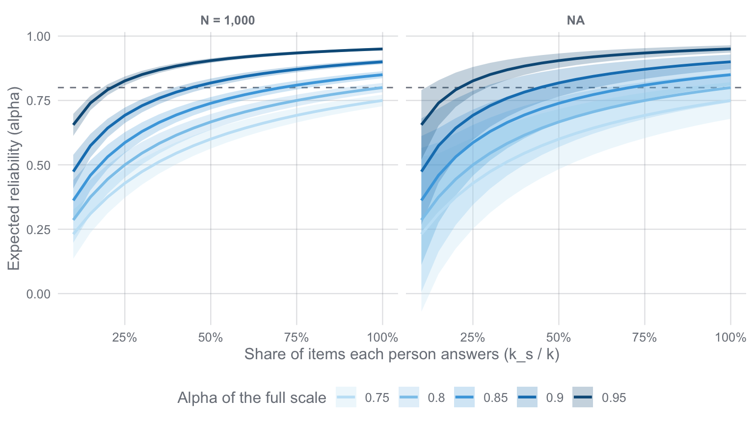

We can see that the ability to “preserve” the reliability drops as the number of items per person decreases. It further decreases faster if the original reliability was already low. Yet, there are some interesting insights here: For example, if the original reliability is .9, we can “afford” up to 50% missings per person and still end up with a reliability of .80. If we only use a third of the items, we can still reach reliabilities of .75, which again may be acceptable in some contexts. The sample size does not change these expected values, it only affects how precisely we can estimate them.

ggplot(analytic, aes(n, r, colour = factor(alpha), fill = factor(alpha))) +
  geom_hline(yintercept = c(.8, .9), linetype = "dashed", colour = "#8a8f98") +
  geom_ribbon(aes(ymin = r - 1.96 * se_r, ymax = pmin(1, r + 1.96 * se_r)), alpha = .25, colour = NA) +
  geom_line(linewidth = 1) +
  facet_wrap(~ N) +
  scale_colour_manual(values = blues) +
  scale_fill_manual(values = blues) +
  scale_x_continuous(labels = scales::percent) +
  labs(x = "Share of items each person answers (k_s / k)",
       y = "Expected correlation with the full scale",
       colour = "Alpha of the full scale", fill = "Alpha of the full scale") +
  theme_blog()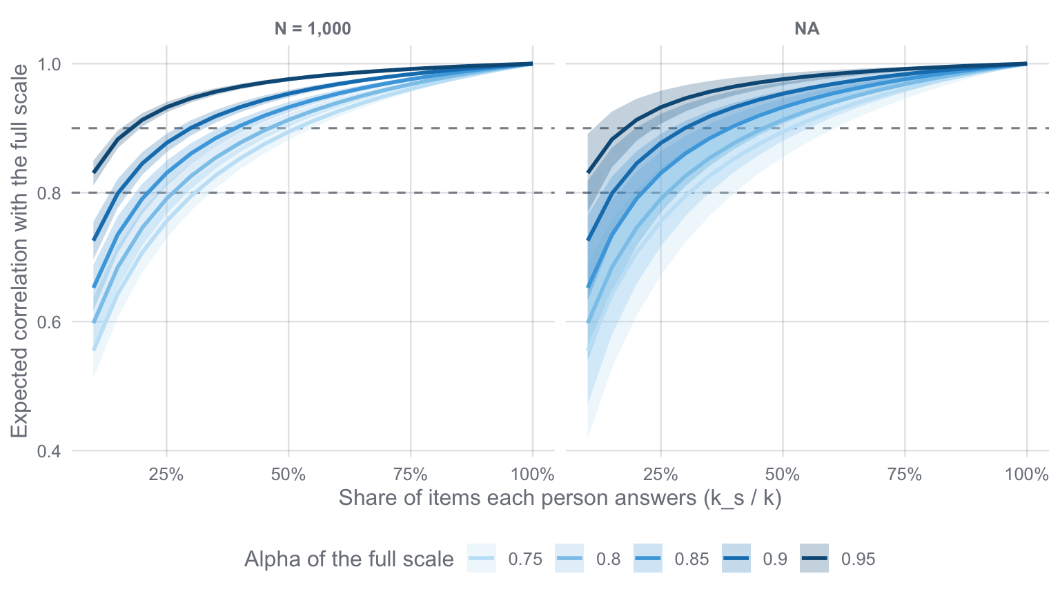

With regard to the validity of the reduced scale, we can see that for scales with a reliability of at least .8, we can afford up to 50% missings and still have good convergent validity with the full scale (r > .90), and up to 70% missings if a validity of r > .80 is sufficient.

Bear in mind that this is just the result based on the formulas outlined above. Practically, however, more things may have to be taken into account:

• Normal Distribution Assumption: The formulas assume that the underlying data is normally distributed, which might not be the case in reality (e.g., with Likert-type items).
• Equal Item Parameters: The formulas assume that all items have equal difficulty and discrimination parameters, while in reality, items can vary significantly.
• Multidimensionality: Real data might have multiple underlying factors, while the theoretical formula assumes unidimensionality.
• Nonlinear Relationships: Real data might include non-linear relationships between items and the latent trait, which are not considered in the formulas.
• Sampling Variability: In real data, there is inherent variability due to random sampling. This can lead to differences between theoretical expectations and observed outcomes.
• Computation of the scales’ scores: The way we handle the missing items when computing each person’s score could significantly impact the results.

To explore these issues a bit further, let’s simulate some data and introduce missings per person systematically.

Simulation approach

The key idea of the simulation is to generate data for which we know each person’s true score. Then we can measure directly how well the scores based on the sampled items recover it: the squared correlation between a score and the true score is exactly the reliability of that score. This is the same quantity the Spearman–Brown formula predicts, so we can compare the two.

library(lavaan)
library(mice)
library(furrr)

Simulating Likert-type items with known true scores

I simulate items from a one-factor model. First, I compute the average inter-item correlation that corresponds to the alpha level we are providing, and from it the factor loading of each item. Each person gets a true score \(\theta\), and each item response is \(\lambda\theta\) plus random error. To make the data look like a typical questionnaire, I cut the responses into 5 answer options. Because real items also differ in how easy they are to agree with, each item gets its own difficulty (a shift of the answer thresholds).

set.seed(123)  # for reproducibility

sim_items <- function(N, k, alpha, answer_options = 5) {

  # Average inter-item correlation implied by alpha, and the resulting loading
  rbar   <- alpha / (k - alpha * (k - 1))
  lambda <- sqrt(rbar)

  # True scores, item difficulties and continuous responses
  theta      <- rnorm(N)
  difficulty <- runif(k, -.75, .75)
  latent <- theta %o% rep(lambda, k) +
    matrix(rnorm(N * k, sd = sqrt(1 - lambda^2)), N, k) -
    matrix(difficulty, N, k, byrow = TRUE)

  # Cut into Likert-type answer options (1 to 5)
  cuts  <- qnorm(seq(0, 1, length.out = answer_options + 1))[2:answer_options]
  items <- matrix(findInterval(latent, cuts) + 1, N, k,
                  dimnames = list(NULL, paste0("i", 1:k)))

  list(items = as.data.frame(items), theta = theta)
}

# Check function
test <- sim_items(N = 100, k = 10, alpha = .9)
head(test$items)

#>   i1 i2 i3 i4 i5 i6 i7 i8 i9 i10
#> 1  3  1  2  1  2  1  3  3  2   5
#> 2  2  1  1  2  2  1  4  3  5   4
#> 3  4  3  5  5  2  2  4  5  5   5
#> 4  3  4  4  2  4  2  4  4  4   5
#> 5  5  2  5  3  3  1  4  4  4   4
#> 6  5  4  5  5  5  4  5  2  5   5

As we can see, the function creates a data set with 10 items and n = 100 participants. Let’s check the alpha level of this scale:

psych::alpha(test$items)$total

#>  raw_alpha std.alpha   G6(smc) average_r     S/N        ase  mean        sd
#>  0.8482603 0.8487234 0.8451815 0.3594018 5.61041 0.02258244 3.164 0.8487091
#>   median_r
#>  0.3625075

It is slightly lower than the specified .90. Cutting continuous responses into five categories always loses a bit of information. That’s why the simulation below compares everything with the alpha of the simulated (Likert-type) data, not with the input value.

Introducing item sampling

Next, we need a function that simulates the item sampling procedure. A random item sampling procedure is the same as introducing a certain number of missings per person (i.e., per row): for each person, only a random subset of round(n * k) items is kept.

sample_items <- function(items, n) {
  k   <- ncol(items)
  k_s <- round(n * k)
  for (i in seq_len(nrow(items))) {
    items[i, sample(k, k - k_s)] <- NA
  }
  items
}

# Check function
test_na <- sample_items(test$items, n = .8)
head(test_na)

#>   i1 i2 i3 i4 i5 i6 i7 i8 i9 i10
#> 1  3  1  2  1 NA  1  3 NA  2   5
#> 2  2  1 NA  2  2  1 NA  3  5   4
#> 3  4  3  5  5  2 NA  4 NA  5   5
#> 4  3  4  4  2  4 NA  4  4  4  NA
#> 5  5  2  5  3  3  1  4 NA  4  NA
#> 6  5  4  5  5  5 NA  5  2  5  NA

Here, I sample 80% of the items per person (i.e., 2 of the 10 items are missing). In fact, this corresponds to an overall amount of missings in the data set of 20%:

mean(is.na(test_na))

#> [1] 0.2

Three ways to score item-sampled data

How do we compute a score for each person if everyone answered different items? I compare three approaches:

1. Mean of the answered items. The simplest option, and probably the most common in practice.
2. Difficulty-adjusted mean. Each item is first centered at its sample mean, then the answered items are averaged. This way, a person who happened to get “easy” items is not advantaged. Under a one-factor model with equal loadings, this is equivalent to a model-based score estimated from the answered items (e.g., a FIML factor score).
3. Imputation first. The unanswered items are imputed (one imputation with predictive mean matching, as implemented in mice), and factor scores are then computed from a CFA on the completed data.

score_mean <- function(items) rowMeans(items, na.rm = TRUE)

score_adjusted <- function(items) {
  centered <- sweep(as.matrix(items), 2, colMeans(items, na.rm = TRUE))
  rowMeans(centered, na.rm = TRUE)
}

score_cfa <- function(items) {
  model <- paste("G =~", paste(names(items), collapse = " + "))
  scores <- as.numeric(lavPredict(cfa(model, data = items, std.lv = TRUE)))
  # The sign of a factor is arbitrary: align it with the sum score
  # (all items are positively keyed)
  if (cor(scores, rowSums(items)) < 0) scores <- -scores
  scores
}

score_imputed <- function(items) {
  score_cfa(complete(mice(items, m = 1, printFlag = FALSE)))
}

# Reliability of each score = squared correlation with the true score
sapply(list(mean     = score_mean(test_na),
            adjusted = score_adjusted(test_na),
            imputed  = score_imputed(test_na)),
       \(score) cor(score, test$theta)^2) |> round(2)

#>     mean adjusted  imputed 
#>     0.79     0.80     0.76

Putting it all together

Now, we put it all together in one function that simulates a data set, samples the items, scores the data in all three ways, and computes two outcomes for each score:

• its reliability: the squared correlation with the true score, and
• its convergent validity: the correlation with the score based on all items (the full-data mean for the two mean-based scores, the full-data factor score for the imputation approach).

It also stores the alpha of the full simulated scale and the reliability the Spearman–Brown formula predicts from it.

alpha_full <- function(items) {
  k <- ncol(items)
  k / (k - 1) * (1 - sum(apply(items, 2, var)) / var(rowSums(items)))
}

sim_func <- function(N, k, alpha, n) {
  d <- sim_items(N, k, alpha)
  sampled <- sample_items(d$items, n)
  a <- alpha_full(d$items)

  full <- list(mean = score_mean(d$items), adjusted = score_mean(d$items),
               imputed = score_cfa(d$items))
  part <- list(mean = score_mean(sampled), adjusted = score_adjusted(sampled),
               imputed = score_imputed(sampled))

  tibble(N = N, k = k, k_s = round(n * k), n = n, alpha = alpha, alpha_emp = a,
         method = names(part),
         r_full = mapply(cor, part, full),
         reliability = sapply(part, cor, y = d$theta)^2,
         reliability_full = sapply(full, cor, y = d$theta)^2,
         spearman_brown = n * a / (1 + (n - 1) * a))
}

# Check sim function
sim_func(N = 500, k = 20, alpha = .85, n = .5)

#> # A tibble: 3 × 11
#>       N     k   k_s     n alpha alpha_emp method   r_full reliability
#>   <dbl> <dbl> <dbl> <dbl> <dbl>     <dbl> <chr>     <dbl>       <dbl>
#> 1   500    20    10   0.5  0.85     0.823 mean      0.912       0.684
#> 2   500    20    10   0.5  0.85     0.823 adjusted  0.926       0.707
#> 3   500    20    10   0.5  0.85     0.823 imputed   0.858       0.607
#> # ℹ 2 more variables: reliability_full <dbl>, spearman_brown <dbl>

We set up a grid that contains the parameter ranges we want to explore and run the function 200 times for each of the 270 combinations. That is 54,000 simulated data sets, each scored in three ways. I use the package furrr to parallelize the procedure; furrr_options(seed = ...) makes the parallel random numbers reproducible.

# Setup simulation grid
setup <- expand.grid(
  N = c(250, 500, 1000),
  k = c(10, 20, 40),
  alpha = seq(.75, .95, by = .05),
  n = c(.3, .4, .5, .6, .7, .8)
)

# The simulation takes a while: its results are saved next to this post and
# re-used (delete sims/results.rds to run it again)
n_sim <- 200
if (file.exists("sims/results.rds")) {
  results <- readRDS("sims/results.rds")
} else {
  plan(multisession, workers = parallelly::availableCores(omit = 1))
  results <- setup[rep(seq_len(nrow(setup)), n_sim), ] |>
    future_pmap_dfr(sim_func, .options = furrr_options(seed = 2024))
  dir.create("sims", showWarnings = FALSE)
  saveRDS(results, "sims/results.rds")
}

results

#> # A tibble: 162,000 × 11
#>        N     k   k_s     n alpha alpha_emp method   r_full reliability
#>    <dbl> <dbl> <dbl> <dbl> <dbl>     <dbl> <chr>     <dbl>       <dbl>
#>  1   250    10     3   0.3  0.75     0.771 mean      0.780       0.408
#>  2   250    10     3   0.3  0.75     0.771 adjusted  0.811       0.451
#>  3   250    10     3   0.3  0.75     0.771 imputed   0.647       0.297
#>  4   500    10     3   0.3  0.75     0.718 mean      0.740       0.397
#>  5   500    10     3   0.3  0.75     0.718 adjusted  0.779       0.436
#>  6   500    10     3   0.3  0.75     0.718 imputed   0.508       0.165
#>  7  1000    10     3   0.3  0.75     0.727 mean      0.753       0.410
#>  8  1000    10     3   0.3  0.75     0.727 adjusted  0.781       0.435
#>  9  1000    10     3   0.3  0.75     0.727 imputed   0.597       0.251
#> 10   250    20     6   0.3  0.75     0.741 mean      0.777       0.438
#> # ℹ 161,990 more rows
#> # ℹ 2 more variables: reliability_full <dbl>, spearman_brown <dbl>

Reliability of the item-sampled scores

The first figure shows the reliability of each person’s score, depending on the share of items they answered and the alpha of the full scale (for a sample of 500 and a pool of 20 items). The dashed line is the reliability predicted by the Spearman–Brown formula.

d <- filter(summ, N == 500, k == 20)

ggplot(d, aes(n, rel, colour = method)) +
  geom_line(aes(y = sb), colour = "#8a8f98", linetype = "dashed", linewidth = .8) +
  geom_pointrange(aes(ymin = rel_lo, ymax = rel_hi), size = .2,
                  position = position_dodge(width = .04)) +
  geom_line(position = position_dodge(width = .04)) +
  facet_wrap(~ lab, nrow = 1) +
  scale_colour_manual(values = method_cols, labels = method_labels) +
  scale_x_continuous(labels = scales::percent, breaks = c(.3, .5, .7)) +
  labs(x = "Share of items each person answers",
       y = "Reliability of the person scores",
       colour = NULL,
       caption = "Points: mean of 200 replications, bars: 95% of replications. Dashed: Spearman–Brown prediction.") +
  theme_blog() +
  theme(plot.caption = element_text(colour = "#7a7f88"))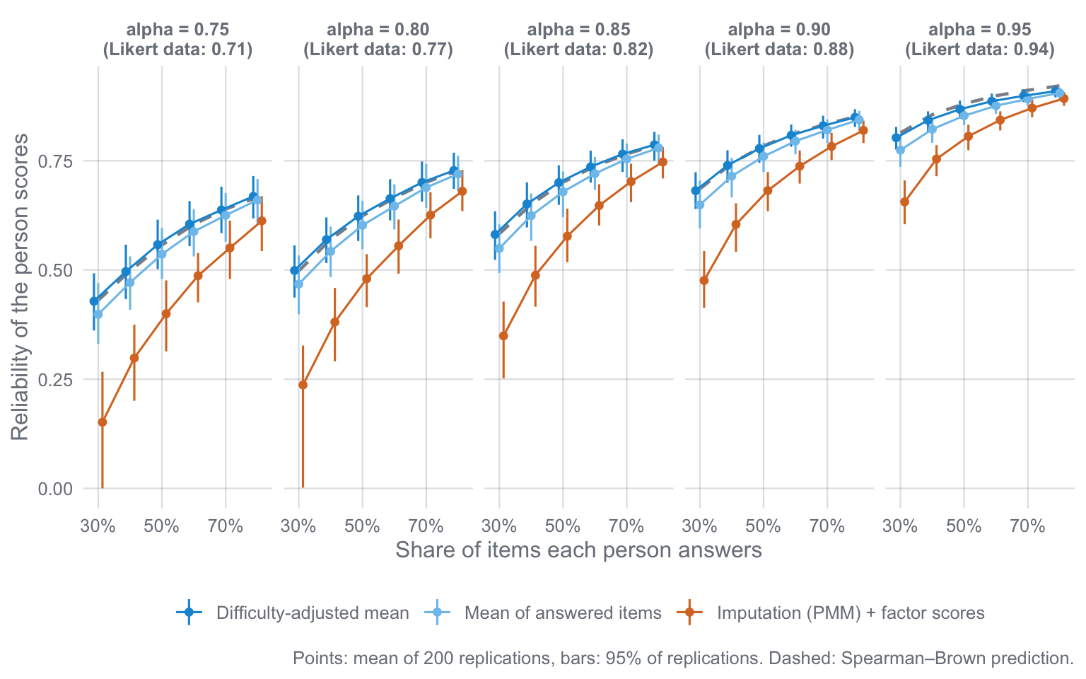

Three things stand out:

1. The Spearman–Brown formula works well. Averaged across all 270 conditions, the reliability of the difficulty-adjusted mean is 0.71, practically identical to the predicted 0.71 (the mean absolute deviation is only 0.005). The simple mean of the answered items is only slightly worse; its small disadvantage comes from items differing in difficulty, so getting “easy” or “hard” items adds a bit of noise.
2. Imputing first makes things worse. Scores based on the imputed data are less reliable in every condition, on average by 0.11 (for N = 500 and k = 20). Imputation cannot add information about a person; it fills in plausible values that include random noise, and that noise ends up in the scores.
3. The loss is largest when few items are answered. It grows from 0.04 when people answer 80% of the items to 0.22 when they answer 30%. For example, with a scale of alpha = .85 and half of the items answered, the reliability is 0.70 for the difficulty-adjusted mean but only 0.58 with imputation.

Correlation with the full scale (convergent validity)

Next, we can look at the correlation between the item-sampled scores and the scores based on all items. The dashed line shows the part–whole correlation expected from the formulas above.

ggplot(d, aes(n, r, colour = method)) +
  geom_line(aes(y = sqrt(sb / alpha_emp)), colour = "#8a8f98", linetype = "dashed", linewidth = .8) +
  geom_hline(yintercept = c(.8, .9), colour = "#8a8f9860") +
  geom_pointrange(aes(ymin = r_lo, ymax = r_hi), size = .2,
                  position = position_dodge(width = .04)) +
  geom_line(position = position_dodge(width = .04)) +
  facet_wrap(~ lab, nrow = 1) +
  scale_colour_manual(values = method_cols, labels = method_labels) +
  scale_x_continuous(labels = scales::percent, breaks = c(.3, .5, .7)) +
  labs(x = "Share of items each person answers",
       y = "Correlation with the full-scale score",
       colour = NULL) +
  theme_blog()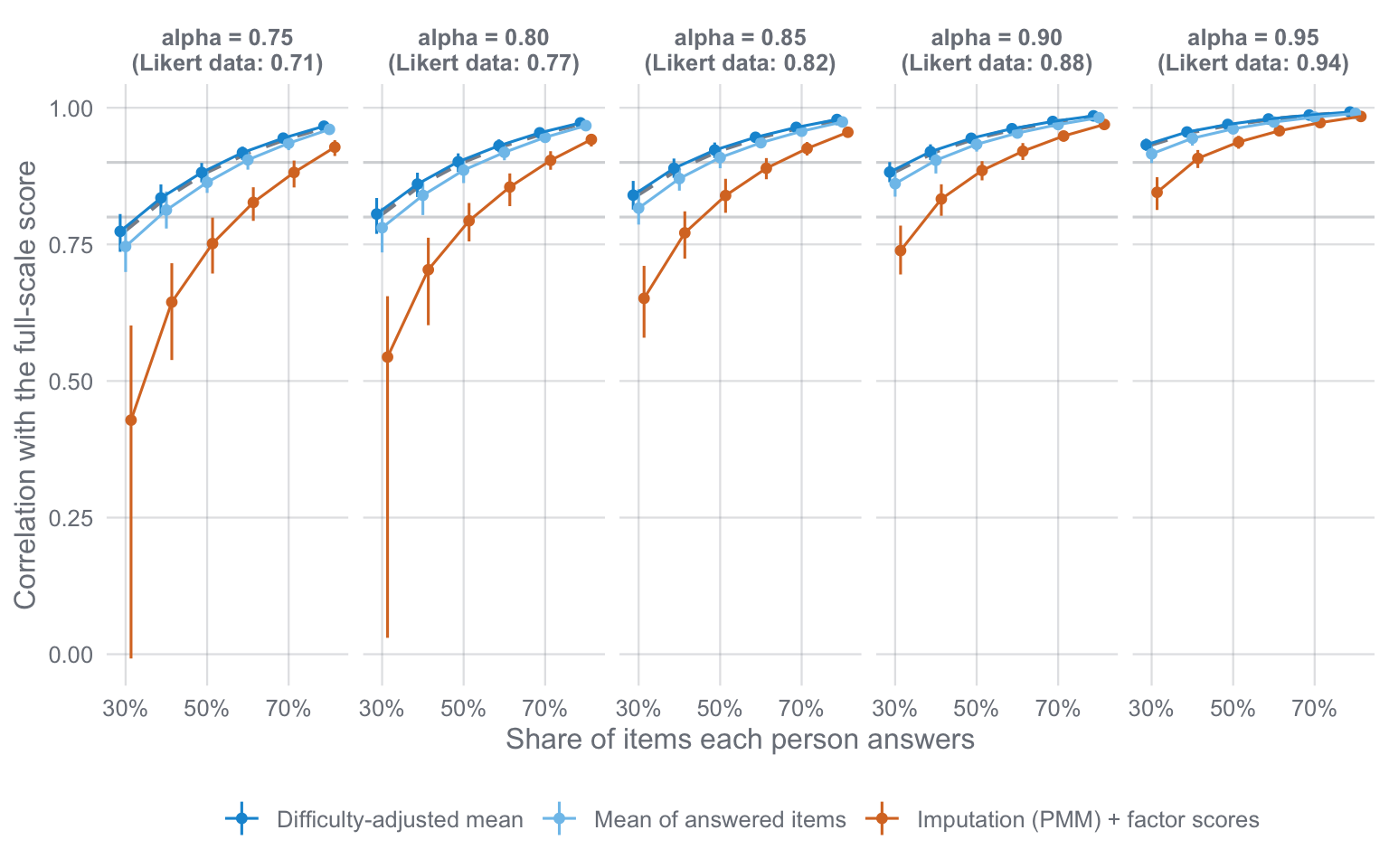

The picture is the same: the mean-based scores correlate with the full-scale scores as expected, the imputation-based scores less so. If the original scale has a high reliability (alpha ≥ .85) and people answer at least half of the items, the item-sampled scores correlate r > .90 with the full scale.

Do sample size and item pool size matter?

Interestingly, sample size and the size of the item pool hardly matter:

summ |>
  filter(method == "adjusted", alpha == .85, n == .5) |>
  ggplot(aes(factor(N), rel, colour = factor(k))) +
  geom_hline(aes(yintercept = mean(sb)), colour = "#8a8f98", linetype = "dashed") +
  geom_pointrange(aes(ymin = rel_lo, ymax = rel_hi), position = position_dodge(width = .5)) +
  scale_colour_manual(values = c("10" = "#8cc8ec", "20" = "#1497d6", "40" = "#0b5a87")) +
  labs(x = "Sample size", y = "Reliability", colour = "Items in the pool") +
  theme_blog()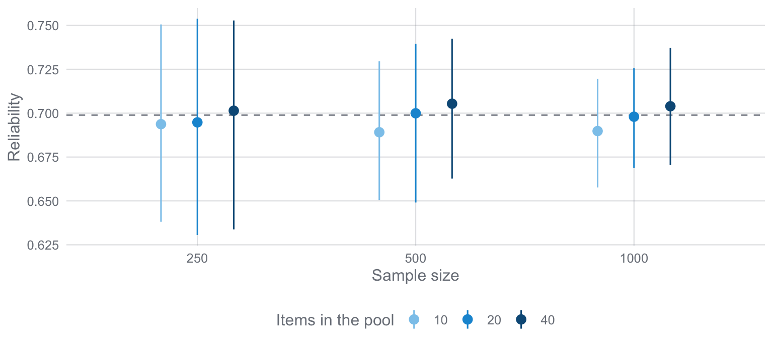

For a given alpha of the full scale and a given share of items answered, the expected reliability is the same for 250 or 1,000 respondents and for pools of 10 or 40 items. A larger sample only makes the result less variable. (Note that in this simulation, a larger pool with the same alpha means weaker individual items. In practice, extending a scale usually increases its alpha, and then a larger pool does help.)

So how does the simulation compare to the mathematical approach outlined above?

Let’s look at one example (N = 500, k = 20, 12 sampled items, alpha = .80):

summ |>
  filter(N == 500, k == 20, n == .6, alpha == .8) |>
  mutate(method = method_labels[as.character(method)]) |>
  select(method, alpha_emp, `Spearman-Brown` = sb, reliability = rel, r_full = r)

#> # A tibble: 3 × 5
#>   method                           alpha_emp `Spearman-Brown` reliability r_full
#>   <chr>                                <dbl>            <dbl>       <dbl>  <dbl>
#> 1 Difficulty-adjusted mean             0.768            0.665       0.663  0.931
#> 2 Imputation (PMM) + factor scores     0.768            0.665       0.555  0.855
#> 3 Mean of answered items               0.768            0.665       0.646  0.918

# Mathematical results (with the alpha of the simulated Likert-type data)
a <- unique(round(filter(summ, N == 500, k == 20, n == .6, alpha == .8)$alpha_emp, 3))
reli_new(alpha = a, k_s = 12, k = 20, N = 500) |>
  mutate(ll = r - 1.96*se_r,
         ul = r + 1.96*se_r) |>
  dplyr::select(N, k, k_s, alpha, alpha_new, r, ll, ul)

#> # A tibble: 1 × 8
#>       N     k   k_s alpha alpha_new     r    ll    ul
#>   <dbl> <dbl> <dbl> <dbl>     <dbl> <dbl> <dbl> <dbl>
#> 1   500    20    12 0.768     0.665 0.931 0.919 0.942

When we measure reliability as the precision of the person scores and use the alpha of the simulated Likert-type data, the simulation and the mathematical approach agree closely for the two mean-based scores.

Conclusion and recommendations

So what does this all mean? From my point of view, the simulations indicate that item sampling is a viable strategy for efficiently measuring latent traits in social science research (e.g., scales of 10-40 items with Likert-type items):

• The Spearman–Brown formula is a good planning tool. Given the alpha of the full scale and the share of items each person answers, it predicts the reliability of the person scores well. Just make sure to plug in the alpha of your actual (Likert-type) data. If the full scale has an alpha of about .90 and people answer half of the items, their scores still have a reliability of about 0.78 and correlate r = 0.94 with the full-scale scores. With a full-scale alpha of .80 to .85, half of the items yields reliabilities of only about 0.62 to 0.70; to reach .80, people then need to answer most of the items.
• Score people on the items they answered; don’t impute. A (difficulty-adjusted) mean or a model-based score from the answered items (e.g., FIML or IRT) is clearly better than imputing the missing items first. Imputation makes the data set look complete, but it adds noise to every person’s score.
• Sample size is about precision, not about reliability. Larger samples estimate everything more precisely, but they do not make each person’s score more reliable.

This technique reduces respondent burden and shortens questionnaires. At the level of the sample (e.g., means and correlations of the scale), item sampling preserves the information of the full item pool. At the level of individuals, the reliability of their scores follows Spearman–Brown, and that is something we can plan for.

References

• de Vet, H. C., Mokkink, L. B., Mosmuller, D. G., & Terwee, C. B. (2017). Spearman–Brown prophecy formula and Cronbach’s alpha: different faces of reliability and opportunities for new applications. Journal of Clinical Epidemiology, 85, 45-49.
• Husek, T. R, & Sirotnik, K. (1967). Item Sampling in Educational Research. https://files.eric.ed.gov/fulltext/ED013975.pdf
• van Zyl, J. M., Neudecker, H., & Nel, D. G. (2000). On the distribution of the maximum likelihood estimator of Cronbach’s alpha. Psychometrika, 65(3), 271-280.

sessionInfo()

#> R version 4.4.0 (2024-04-24)
#> Platform: aarch64-apple-darwin20
#> Running under: macOS 26.6.2
#> 
#> Matrix products: default
#> BLAS:   /Library/Frameworks/R.framework/Versions/4.4-arm64/Resources/lib/libRblas.0.dylib 
#> LAPACK: /Library/Frameworks/R.framework/Versions/4.4-arm64/Resources/lib/libRlapack.dylib;  LAPACK version 3.12.0
#> 
#> locale:
#> [1] C.UTF-8/C.UTF-8/C.UTF-8/C/C.UTF-8/C.UTF-8
#> 
#> time zone: Europe/Amsterdam
#> tzcode source: internal
#> 
#> attached base packages:
#> [1] stats     graphics  grDevices utils     datasets  methods   base     
#> 
#> other attached packages:
#>  [1] furrr_0.3.1     future_1.70.0   mice_3.16.0     lavaan_0.6-19  
#>  [5] lubridate_1.9.3 forcats_1.0.0   stringr_1.6.0   dplyr_1.2.0    
#>  [9] purrr_1.2.1     readr_2.1.5     tidyr_1.3.2     tibble_3.3.1   
#> [13] ggplot2_4.0.2   tidyverse_2.0.0
#> 
#> loaded via a namespace (and not attached):
#>  [1] gtable_0.3.6       shape_1.4.6.1      xfun_0.57          htmlwidgets_1.6.4 
#>  [5] psych_2.4.3        lattice_0.22-6     tzdb_0.4.0         quadprog_1.5-8    
#>  [9] vctrs_0.7.2        tools_4.4.0        Rdpack_2.6.6       generics_0.1.4    
#> [13] parallel_4.4.0     stats4_4.4.0       pan_1.9            pkgconfig_2.0.3   
#> [17] jomo_2.7-6         Matrix_1.7-0       RColorBrewer_1.1-3 S7_0.2.1          
#> [21] lifecycle_1.0.5    compiler_4.4.0     farver_2.1.2       mnormt_2.1.1      
#> [25] codetools_0.2-20   htmltools_0.5.8.1  yaml_2.3.12        glmnet_4.1-8      
#> [29] nloptr_2.2.1       pillar_1.11.1      MASS_7.3-60.2      reformulas_0.4.4  
#> [33] iterators_1.0.14   rpart_4.1.23       boot_1.3-30        foreach_1.5.2     
#> [37] mitml_0.4-5        parallelly_1.46.1  nlme_3.1-164       tidyselect_1.2.1  
#> [41] digest_0.6.39      stringi_1.8.7      listenv_0.10.1     labeling_0.4.3    
#> [45] splines_4.4.0      fastmap_1.2.0      grid_4.4.0         cli_3.6.5         
#> [49] magrittr_2.0.4     utf8_1.2.6         survival_3.5-8     broom_1.0.12      
#> [53] pbivnorm_0.6.0     withr_3.0.2        scales_1.4.0       backports_1.5.0   
#> [57] timechange_0.3.0   rmarkdown_2.30     globals_0.19.1     nnet_7.3-19       
#> [61] lme4_2.0-1         hms_1.1.3          evaluate_1.0.5     knitr_1.51        
#> [65] rbibutils_2.4.1    rlang_1.1.7        Rcpp_1.1.1         glue_1.8.0        
#> [69] minqa_1.2.8        jsonlite_2.0.0     R6_2.6.1